Using the matRad.m script
To execute the matRad script using MATLAB you need to:
If you prefer to only use the GUI to execute matRad, check out the Running the graphical user interface.
Step 1: Open matRad folder in MATLAB
To use matRad you need to open the matRad folder in MATLAB.
Open MATLAB and navigate to the location of the files; if you have cloned the repository, it is most likely located in your local Github folder (e.g. C:\Users\username\Documents\GitHub\matRad).
Inside the matRad folder there are several MATLAB functions used to run matRad, named matRad*.m, and *.mat files containing base data and exemplary patient data sets.
The main script to run matRad is called matRad.m. It can be executed section by section.
Tip
While editing the matrad.m file seems like a good starting point, it is advisable to not touch the original file and git status of the versioned source code. Therefore, you can copy and paste the file into userdata/scripts, as the userdata subfolder is ignored by git.
Step 2: Set patient-specific parameters
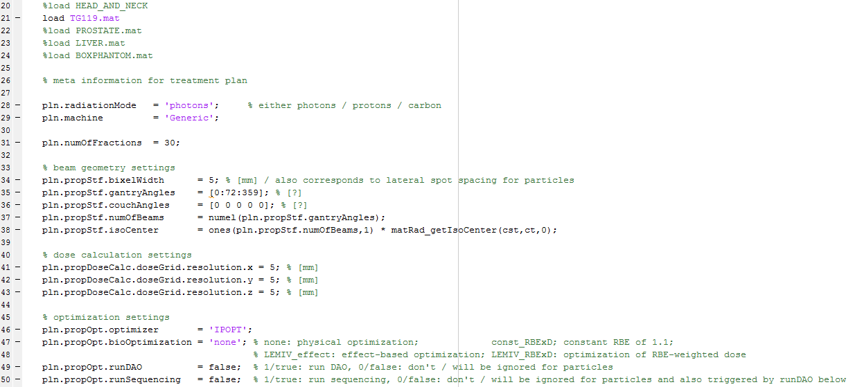
In the first section, the patient specific parameters have to be set (see the parameters screenshot):
1. Selecting a patient
Lines 20-24 in the the parameters screenshot show the patient data sets available by default. Un-comment the data set you wish to use. The dose parameters for the different volumes (min. dose, max. dose, penalties) are set within the patient data set cst cell array. If you wish, you can adjust these parameters before executing matRad.
2. Selecting beam angles
Lines 35-36 in the the parameters screenshot are used to set the gantry and couch angles. Here you can set any angles from 0-359°. Make sure that you always create pairs of gantry and couch angles; otherwise, you won’t be able to execute the inverse planning!
3. Selecting radiation mode
The radiation mode can be set in line 28 in the the parameters screenshot. You can choose between photons, protons and carbon.
If you decide to use protons or carbon, it is possible to set the lateral spot spacing (line 34). When using carbon, you can also choose between a physical optimization ('none'), an optimization of the biological effect ('effect') or an optimization of the RBE-weighted dose ('RBExD') by adjusting the parameter pln.propOpt.bioOptimization in line 47.
In case you choose photons, it is possible to run an additional MLC sequencing by setting pln.propOpt.runSequencing (line 50) and direct aperture optimization is accessible through pln.propOpt.runDAO (line 49).
The desired number of fractions can be set in line 31 in the the parameters screenshot.
The other parameters set in this section are generated automatically and should not be changed.
Screenshot of the parameters section:
Step 3: Execute inverse planning
The matRad.m script can now be executed step by step:
To evaluate a single section, you have to “activate” it (Left-click inside section) and then use ctrl + enter, use Right-click → Run Section or click Run Section within the Editor window of the MATLAB interface.
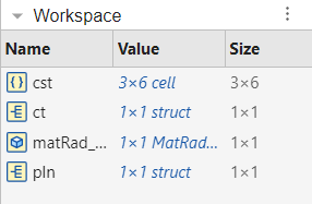
1. Load settings
Now you can execute the first section. You should see, among others, the variables cst, ct and pln in your Workspace.
2. Initial visualization
After the patient data is loaded, you can execute the second section to open the GUI:

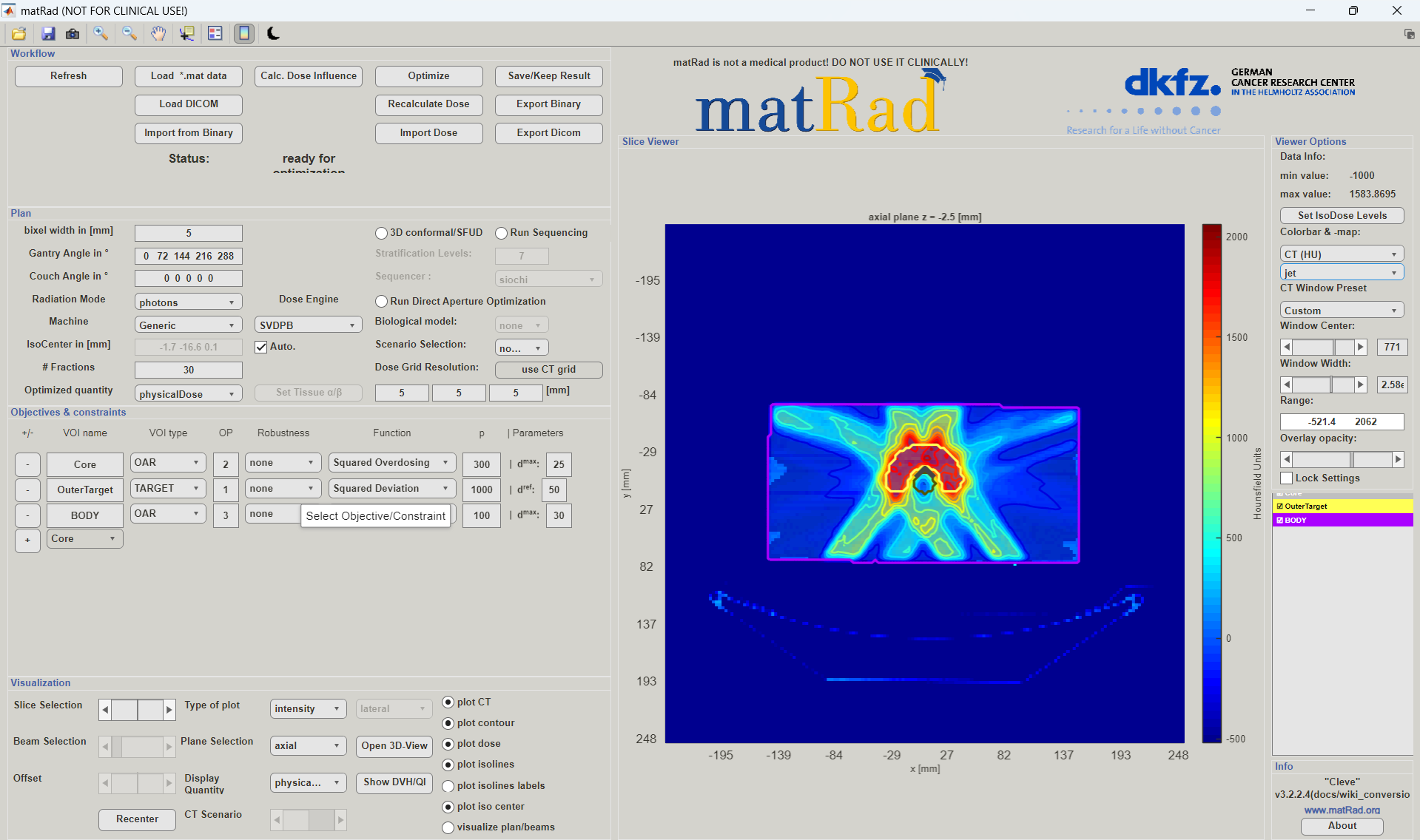
In the GUI you can view the patient CT, change the plan parameters and adjust the optimization parameters.
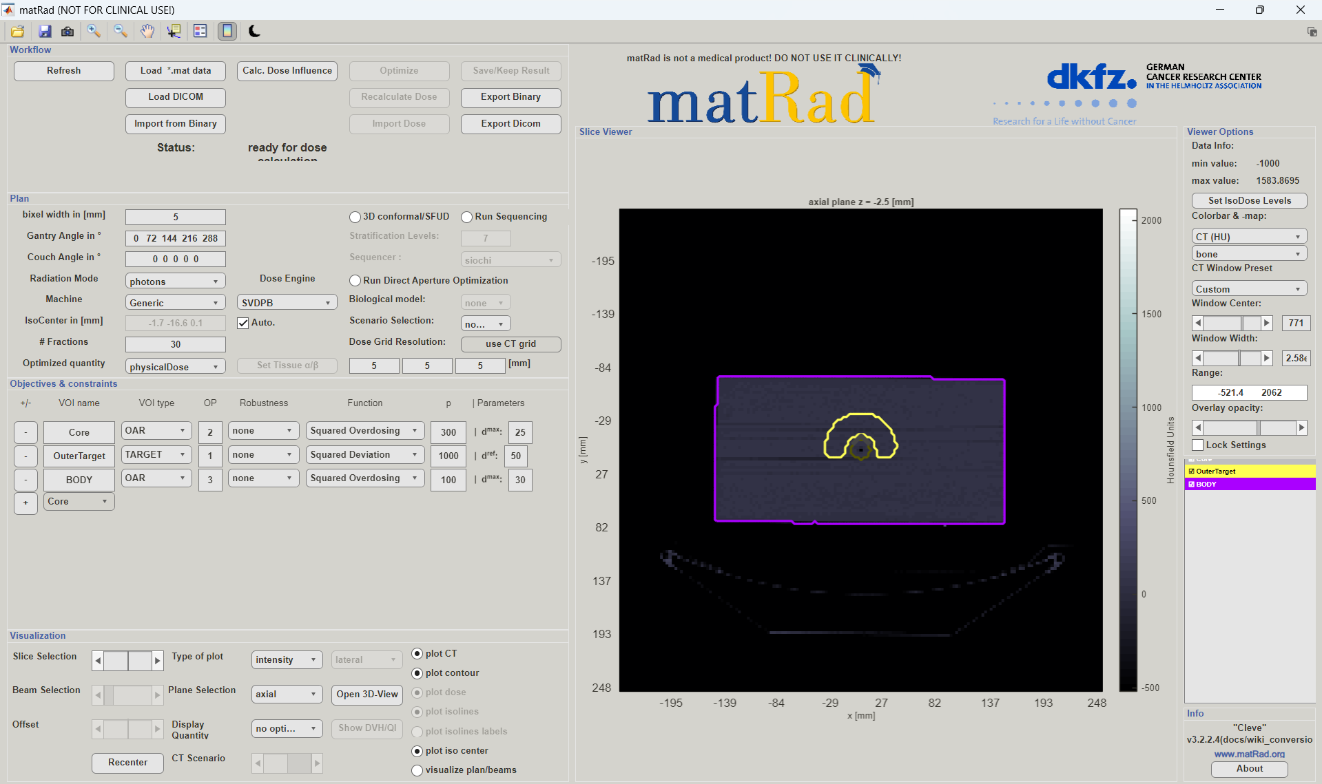
The usage of the GUI is explained in more detail in the Running the graphical user interface. Here we will focus on the “manual” execution of the matRad script. To “manually” change the optimization parameters, you can adjust the cst-cell (see cst cell array documentation for more information).
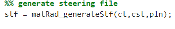
3. Generate steering file
In this section, the steering file stf is created and the matRad steering information is stored as a struct (see stf struct for more information).
The Command Window should show the progress.

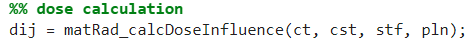
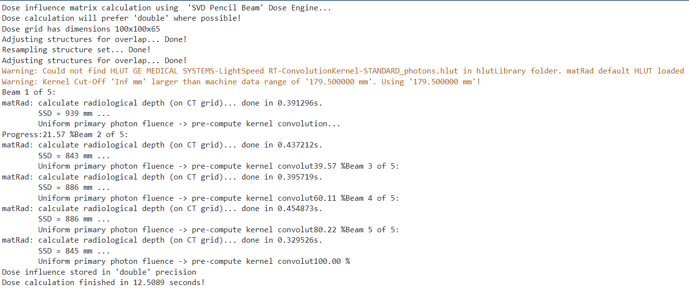
4. Dose calculation
In this section, the dose influence matrix dij for the defined beam angles is calculated (see dij struct for more information).
Again, the progress should be shown in the Command Window.
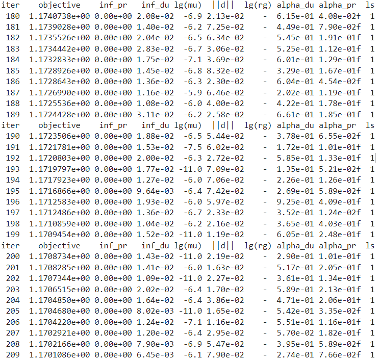
5. Fluence optimization
In this section, the fluence is optimized to find the bixel (photons) or spot (protons/carbon) weights minimizing the objective function.

During this process, the current objective function value is displayed:
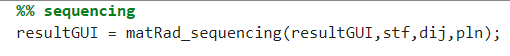
6. Sequencing
For photon IMRT the application of a multileaf collimator is necessary. By sequencing, the applicable dose distribution can be simulated. The fourth input of matRad_engelLeafSequencing(resultGUI,stf,dij,7) is the number of stratification levels. You can adjust this number to use the number of levels you want.
When the sequencing is finished, the result struct is updated.
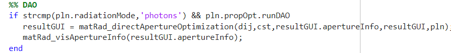
7. Direct aperture optimization
For photon therapy, the multileaf collimator sequencing can be further refined by using an experimental gradient-based direct aperture optimization algorithm, where leaf settings and aperture intensities are optimized simultaneously. Further information including references about the direct aperture optimization algorithm can be found directly in the source code or in the technical documentation about the fluence optimization.
8. Visualization of the resulting treatment plan
Now you can visualize the resulting treatment plan using the GUI.
In the GUI you can see the resulting dose distribution for the calculated treatment plan. You can choose which plane and slice should be displayed. You can also display a dose profile plot by changing Type of plot from intensity to profile. If you have chosen a biological optimization, then you have several parameters to be displayed (e.g. RBE-weighted dose, biological effect, α or β values).
9. Show DVH and quality indicators
In this section, the dose-volume histograms (DVH) are calculated and visualized.

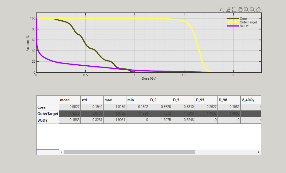
The diagram shows the DVH and in the table, you see the mean, maximum and minimum dose for every VOI. Additionally, the dose and dose-volume coefficient for several confidence levels are displayed.
Step 4: Import additional patient data
matRad supports the import of patient data stored in the DICOM format. A set of functions designed for this purpose can be found in the subfolder dicom. For more information about the usage of the import functions please check out the dicom import page.